Making a Gradebook in Excel
Making a Gradebook in Excel | |
Set Up Your Gradebook An Excel spreadsheet to keep your grades for you is a pretty easy thing to quickly set up, but can save you hours of time later, especially if math was not your favorite subject. 1) Open a blank spreadsheet in Excel. Type the date, term, and course info at the top so you can quickly tell which spreadsheet goes with which class. Next type labels for your assignments across the spreadsheet, and below that the student ID/SSN numbers and names down the first few columns. Leave two blank columns between the students' names and the first assignment column. Use whatever labels you like ("Paper 1 (100)" "Final Project"). 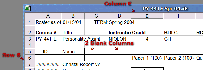 You can use the TAB key to move from column to column. While in a real spreadsheet, the students' SSNs are visible, for security reasons, I've hidden them here. 2) If the cells aren't wide enough to read easily, left click on the first cell (E6 in this case - that's Column E and Row 6) and drag the cursor to the last cell. Then click FORMAT > COLUMN> AUTOFIT to make Excel automatically resize them so you can see all the text in them. 3) Save the file and you're done until you want to enter grades. Entering Grades Entering grades is pretty easy. 1) Open the Excel worksheet, highlight the first cell under the assignment column. In this example, it's E7, Robert's grade for the first paper, and enter the numerical grade. Hit ENTER. This enters the grade and takes you down to the next row. 2) Enter the next grade, and the next, and the next… 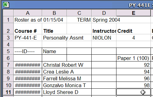 3) Remember how we skipped a column after the student's names? When you are done with entering the grades for this assignment, skip a row, then highlight a cell in the empty column (Column D) and type AVERAGE. 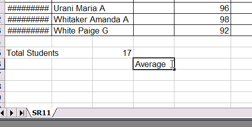 4) Next, select the cell just to the right (in Column E). In the formula box type "=AVERAGE(" then the first cell with grades (E7 in this case) and then a colon (:) and then the last cell with grades (E23 in this case) and finally a ")" -- "=AVERAGE(E7:E23)" will be the final result. That tells Excel to compute an AVERAGE for cells E7 to E23. Hit ENTER to let Excel know you are done with entering the formula and want to see the results.
5) TaDa! You have the Average score for that assignment for the class. Move down a row, and repeat this process with MAX (enter the formula =MAX(E7:E23)) and then MIN (enter the formula =MIN(E7:E23)) and you have the highest and lowest scores too. 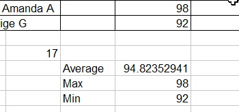 You can enter a formula like this for each column of grades after you've entered them. You can also select the cell with the average, and choose FORMAT > CELLS, the NUMBER tab, and choose NUMBER from the list to make it come out only with two decimal places (94.82) if you are less exact :) You're done! Well, until the next assignment. Keep in mind that a teaching or faculty assistant could do this for you too. Final Grades After all the grades are entered, it's time to let Excel do the math for you. 1) Highlight the cells starting from the first grade, across the row, to the last by left clicking on the first cell and dragging the mouse all the way to the end. You might think it missed the first cell, since it doesn't change color, but don't worry.  2) Look on the toolbar for a button that looks like this  3) You want the total summed for EACH student though, not just the first. Click the total points cell for the first student in the POINTS OBTAINED column. Notice that when you put the cursor over the box, it looks like a fat cross? In the lower right corner of the box is a small square; if you put the cursor over this, it looks like a thin cross.
4) Put the cursor over the little square until you have the thin cross, left click, and drag the cursor down to the last student's row. This highlights the cell in this column for each student in the class. Excel assumes that you made the formula in the first row, and must want it repeated in the other rows. I know the numbers look a litle funny here, but that's because they are made up numbers repeated over and over for students.
5) So you have the total points earned for each student, but you really need the grade earned for each student. Add a label for the next column (column L in this case) like GRADE and then click in the first cell in column L. In the formula bar, type the formula as follows: =K7/460 and then hit ENTER to let Excel know you are done with the formula.
That means "Take the number in K7 and divide by 460". Cell K7 is the cell we made the formula in that sums all points earned. The "/" symbols is for divide, and 460 is the total points possible in this example gradebook. Of course, these will be slightly different for your gradebook, so make sure you reference the right columns for your gradebook. Now you'll get "0.956522" which is fine, but less helpful. Click the cell, and click FORMAT > CELLS, the NUMBER tab, and choose PERCENTAGE from the list. Now the number is formatted like a percentage (95.65%), and is easier to read. Just like before, place the cursor over the small square in the bottom of the cell until you get a thin cross, and drag it down to the last row of students. You'll now have final grade percentages for each student.
Changing Grades Say a student discusses a test question with you and you decide to award her another five points. Simply click her grade, change it, click the mouse in another cell to let Excel know you're done with that cell and want to see the result, and TaDa! The POINTS OBTAINED column and GRADE column are changed automatically. Adding New Assignments Say the class average isn't so good, and several students ask (beg/plead) about adding an extra work assignment. No problem. RIGHT-CLICK the POINTS OBTAINED column, choose INSERT, and a new column is added.
Simply click the cell for the first student in the GRADES column, go to the formula bar, and change the "460" to "472" to change the grade for that student. The final formula looks like this: 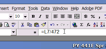 Of course, you want it changed for ALL students, so like before when we copied the formula, put the cursor on the lower right corner of the box until you get a skinny cross, left click, drag the cursor down the column to the last student, and TaDa! Final Grades are updated. A tiny bit trickier is an extra credit assignment. For this, you go to the column after the GRADES column, give it a title like "EXTRA CREDIT", and then enter your grades. Go to the next column, name it something like "NEW GRADE" and click on the first student's cell in the column. Type the following in the formula bar: =(L7+N7)/472 which means "take the number in L7 (which was the total points) and add the number in N7 (the extra credit points), and when done, divide by 472 (the total number of points available without the extra credit). You have to have the parenthesis around the L7+N7 or Excel will divide N7 by 472 and add L7 to the result. 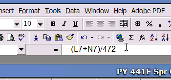 Again, this isn't as helpful, so click the cell, click FORMAT > CELLS, the NUMBER tab, and choose PERCENTAGE from the list. Now the number is formatted like a percentage, and is easier to read. Just like before, place the cursor over the small square in the bottom of the cell until you get a thin cross, and drag it down to the last row of students. You'll now have final final grade percentages for each student. Notice that three students didn't do the assignment. It doesn't change their grade if you just entered a 0.
Adding Comments You might want to save your comments about students with their grades. After the NEW GRADE column, simply add a label of COMMENTS, and type a comment on each student. You might find it annoying to scroll from the far left side of the spreadsheet (where the names are) to the far right (where the comments are). To resolve this, click the ID column and drag the mouse to the NAME column, selecting columns A and B. Then choose WINDOW > FREEZE PANES to make the NAME column stay there at the left margin. 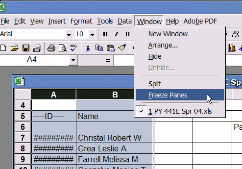  Now scroll right to the COMMENTS column. Notice how the columns go "A, B, C, D, O"? The other columns are still there, and you can see them if you scroll back left, but they are tucked away for right now. If you can't see the comments clearly because they look cut off, highlight the column and choose FORMAT > COLUMN > AUTOFIT SELECTION to make the column the right width. Formatting Want to make it all look pretty? Start at the last row of the last column, and drag the mouse all the way BACK to the first cell in the first column (A1). Then choose FORMAT > AUTOFORMAT and you'll see a list of possible ways Excel can automatically restyle your data. 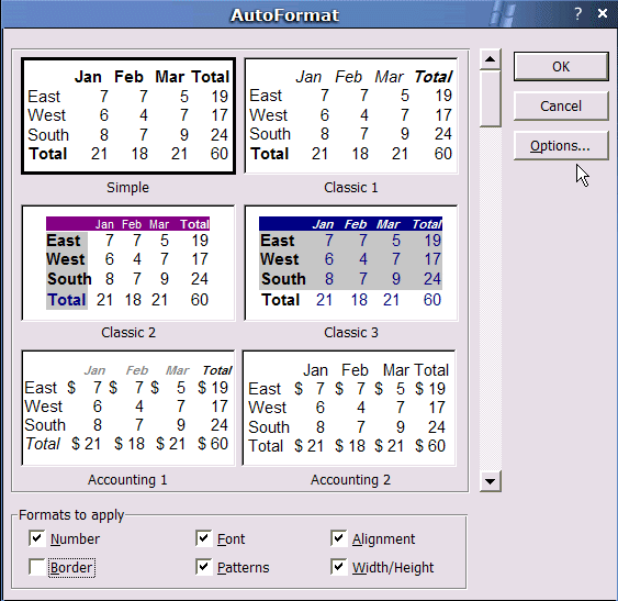 Scroll through the list, click the OPTIONS button on the right to tinker with it a little if you like, and BAM! A totally new look! If you hate it, just hit Ctrl-Z to undo it, or go back to the AUTOFORMAT menu and choose the very last one, which is "None" for no special formatting. 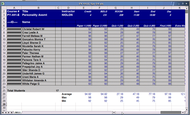 Printing So you want to print out a nice gradesheet, maybe to post on your office door. The problem with this is that you don't want to post student names so everyone sees everyone else's grade, and you don't want to post student SSNs since that presents a risk of identity theft. This isn't as hard as you might think to fix. 1) Go to column C (which we left blank, remember) row 7, which should be right after the first student's name. In the formula bar, type =LEFT(A7,5) which means take the left 5 numbers from column A. Hit ENTER when done. 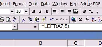 2) As before, select the cell and put the cursor on the box at the lower right corner of the cell until you get the skinny cross, left click and drag to the cell for the last student.
3) LEFT CLICK the A column and drag the cursor to the B column, RIGHT CLICK, and choose HIDE to make these columns disappear. 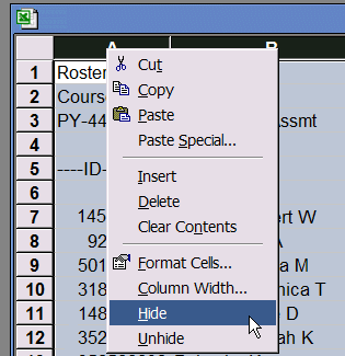 Of course, the columns don't really disappear, they just become 0 inches wide. If you left click on the C column and drag the mouse LEFT, right click again, and choose UNHIDE, it will unhide the columns. 4) Now students can look up their grades by the first five digits of their SSN. The problem now is that anyone could think about the students in the class, and realize alphabetically Robert Christal is likely the top student on the list. Thus, you could figure which grade was his grade pretty easily. To fix this, select the rows with student grades by left clicking the number of the row and dragging the cursor to the last student. 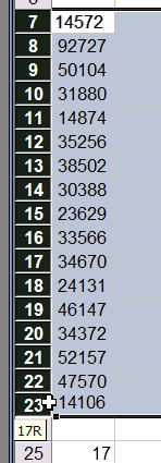 Now choose choose DATA > SORT and have Excel sort these rows by the first five digits of the SSN. 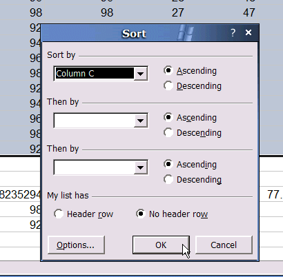 TaDa! Nobody knows who's grade is who's, AND it's easier to find your grade on the sheet! 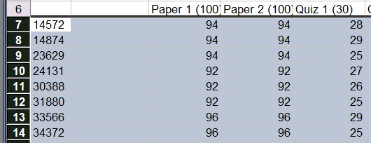 5) Now for printing. Choose FILE > PAGE SETUP and under the PAGE tab choose LANDSCAPE and FIT TO 1 PAGE(S) WIDE as well, and you're ready to print. 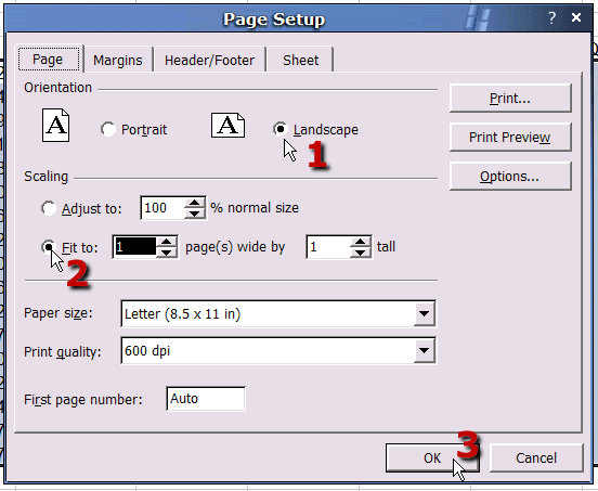 Click OK, and then FILE > PRINT. You can also choose FILE > PRINT PREVIEW to see how it will look first. If it prints out too small, choose the MARGINS tab and make them smaller, or change the FIT TO settings (#2 above). You're Done! One spreadsheet gradebook! |